Recently, I implemented a stratified sampler in my path tracer, following Physically Based Rendering (Pharr et al., 2023, Chapter 8.5). It has the limitation that, unlike the quasi-Monte Carlo samplers in the book, it does not attempt to distribute samples well across pixels, and this is the limitation I want to address.

This is particularly important for low sample count images, and especially real-time rendering. Avoiding clustering (low-frequency noise) in the sample distribution makes denoising easier. I recall most stochastic methods in real-time rendering (e.g. soft shadows, ambient occlusion, screen-space GI) use blue noise textures to offset sample locations in a well-distributed way. I am not sure what the proper citation for this is, but I found (Georgiev & Fajardo, 2016) which describes the method. Regardless, I’m exploring a different approach in this post.

Stratified sampling is a variance reduction technique which divides the integration domain into disjoint regions called strata and places one sample in each of them. For example, to place 16 stratified samples in a unit square, you would overlay a \(4 \times 4\) grid and place one sample in each grid cell. It is important to randomise the location of the sample within each stratum (jitter) so that undersampled details become noise, rather than aliasing.

Stratifying a high-dimensional integration domain requires a sample count exponential in the number of dimensions. For the light transport problem, this is infeasible, so instead the stratified sampler pairs up dimensions used together (e.g. for BSDF sampling), and each group is independently stratified. To avoid undesired correlations between dimensions and between pixels, the order in which strata receive samples is randomised using the hash of the pixel coordinates and the dimension.

The more sophisticated samplers that the PBR book describes, which are based on deterministic low-discrepancy sequences, produce samples which are well-distributed over all dimensions simultaneously. This makes it fairly straightforward to make the samples in a pixel well-distributed with respect to neighbouring pixels: you just stretch the first two dimensions across the pixel grid. However, doing this with the stratified sampler is completely useless¹ because, as discussed before, each pair of dimensions are independent of each other.

The main constraint I had when considering how to improve the cross-pixel distribution was that the stratification of individual pixels needed to be unchanged, so that the convergence rate of each pixel is not harmed. If I render an image with 16spp, then whatever solution I come up with must still put one sample in each of the \(4 \times 4\) grid cells. Approaches such as using a single permutation for a group of pixels don’t work since you can’t guarantee that the pixels end up stratified, only that the group is, at least with how I choose permutations.

The solution I came up with is to stratify the random jitter within each stratum across pixels. The stratum in which to place the sample is first selected in the normal way, so that the individual pixel distribution is not impacted. Then, a 4-element permutation is selected by hashing the coordinates of the \(2 \times 2\) image tile, the selected stratum, and the dimension. This permutation is indexed using the pixel coordinate within the \(2 \times 2\) image tile. Below is the resulting sample distribution in a \(2 \times 2\) image tile with 16spp, with each sample point coloured according to which pixel they belong to.

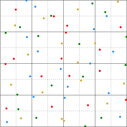
Each pixel still gets samples stratified in a \(4 \times 4\) grid (as required), while the whole tile gets samples stratified in an \(8 \times 8\) grid. In the case that the pixels are highly correlated, for example when the camera rays all land next to each other, this effectively filters out low-frequency noise. The improvement in image quality is only obvious at very low sample counts, so here is a 4 sample per pixel render of my version of the Cornell Box scene²:

Baseline

2x2 Stratification

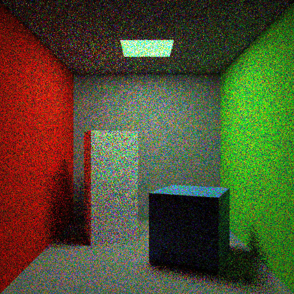
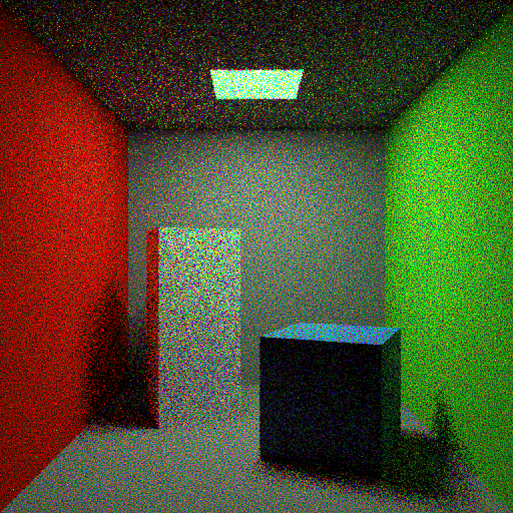
The baseline image has a lot of clustering; you can see large groups of pixels similarly shaded on every directly lit surface. The new image has very little clustering in comparison, which looks much better. Of course, the numeric error is the same, since only the image-space distribution of the error has changed.

This process can be iterated to stratify the jitter locations within the jittered stratum. It should be obvious that it’s most important for nearby pixels to have the largest difference in sample positions, so each iteration distributes samples into smaller stratum which are distributed across a larger area. The pseudocode for this is:

1
2
3
4
5
6
7
8
9
10
11
12
13
14
15
16
17
18
def sample_stratum(pixel: ivec2, sample: int, dimension: int, sqrt_spp: int) -> vec2:
    stratum: ivec2 = pick_stratum(sample, sqrt_spp, hash(pixel, dimension))

    for i in range(JITTERS) {
        tile = (pixel >> i) // 2;
        subtile = (pixel >> i) % 2;
        key = hash(tile, dimension, stratum, i);
        jitter_stratum = pick_stratum(subtile.x + 2 * subtile.y, 2, key)
        stratum = 2 * stratum + jitter_stratum
    }

    # Jitter in final stratum and scale to [0, 1)
    return (stratum + random()) / (sqrt_spp << JITTERS)

def pick_stratum(index: int, sqrt_n: int, key: int) -> ivec2:
    # Use permutation to select grid cell, and returned unscaled stratum vector
    idx = permutation_element(index, sqrt_n**2, key)
    return ivec2(idx % sqrt_n, idx // sqrt_n)

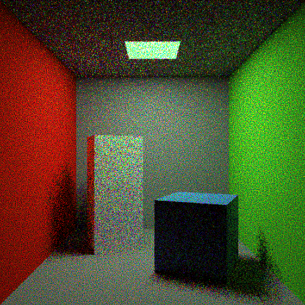
Here is the same scene from before, comparing one iteration (i.e. the \(2 \times 2\) stratification above) to 8 iterations. The improvement from the additional iterations is not as obvious, but is still clearly there.

1 Iteration

8 Iterations

For actual scenes, rendered with vaguely reasonable sample counts, the improvement ranges from “subtle” to “nonexistent”. Here is the Salle de bain scene by nacimus from Benedikt Bitterli’s Rendering Resources (Bitterli, 2016), rendered with 64 samples per pixel³:

Baseline

Cross-pixel Stratification

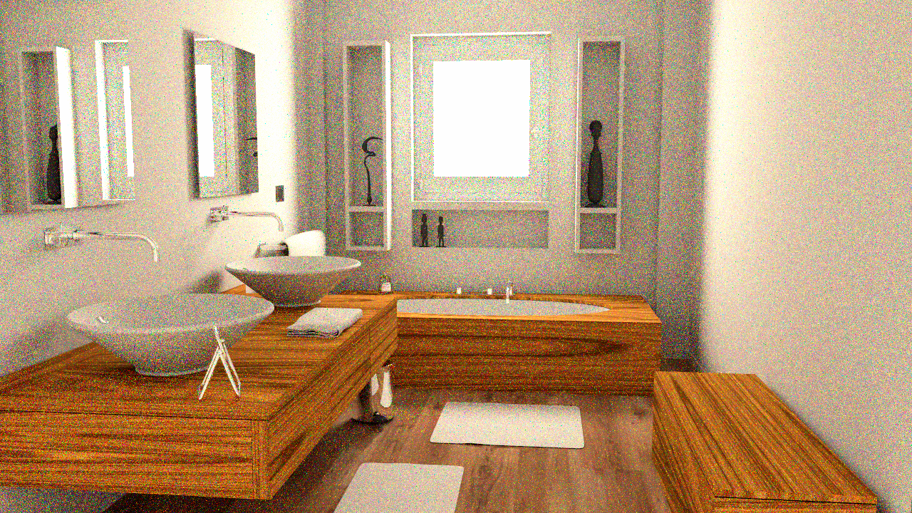
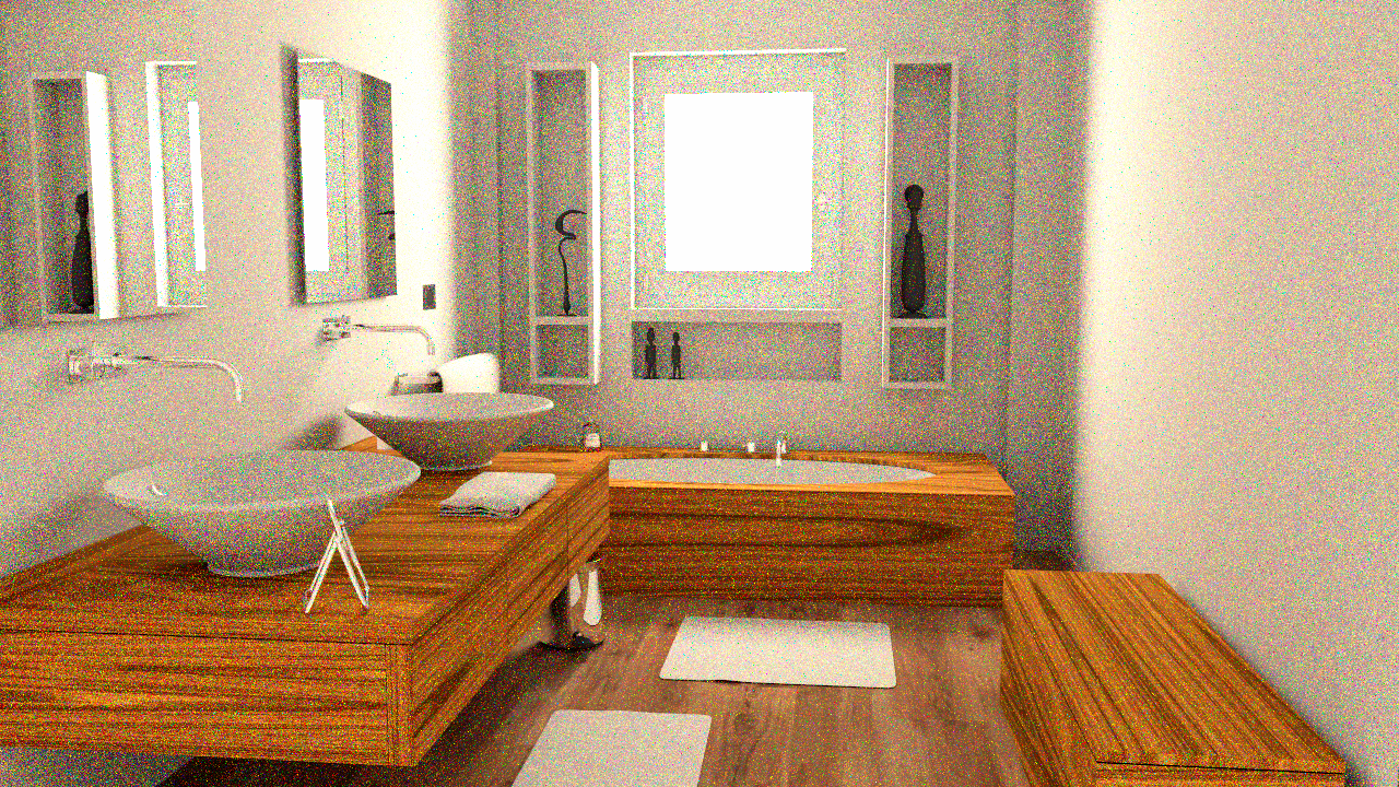
I think this is improved by the cross-pixel stratification, but only a little.

Of course, the quasi-Monte Carlo samplers (which I can’t compare against because I haven’t implemented them) are obviously much better, as they can simultaneously distribute samples well across all dimensions and across pixels, and I believe partial renders also get well-distributed samples. For the basic stratified sampler, only the final image uses well-distributed samples; intermediate results (preview images) are not much different from independent sampling, and this cross-pixel stratification scheme doesn’t help with that.

Overall, this technique has limited utility since better options (quasi-Monte Carlo and blue noise dithered sampling) exist. Its only real advantage is that it’s an easily implemented extension to an existing stratified sampling implementation. It was fun to think about and come up with though, and that’s all that really matters in the end!

References

1. Pharr, M., Humphreys, G., Raghavachary, S., & Hanrahan, P. (2023). Physically based rendering. The MIT Press. https://pbr-book.org/
2. Georgiev, I., & Fajardo, M. (2016). Blue-noise dithered sampling. In ACM SIGGRAPH 2016 Talks (pp. 1–1).
3. Bitterli, B. (2016). Rendering resources. https://benedikt-bitterli.me/resources/